I’ve spent over a decade working with BigQuery, watching it mature through many feature releases. It abstracts away an enormous amount of complexity, but not all of it. If you have spent any time in the real world with it, you have met the standard BigQuery query optimization checklists. Name your columns instead of using SELECT *. Filter on the partition column. Avoid CTEs. Cast your join keys.
You nod, refactor your SQL, and check the results. Sometimes nothing happens. Sometimes the execution time drops but the billed cost stays exactly the same. In the worst cases you waste hours on a recommendation that does not apply to your environment.
Generic advice treats all optimizations as equal. They aren’t. Here is what “BigQuery Query Optimization” means in this article:
Implementing query optimizations in BigQuery that actually save you money and improve performance requires understanding five layers and the most effective query optimization techniques: partition pruning, column pruning, sampling and sketches, result caching, history-based optimizations, materialized views, data models and storage optimization. In this article, I include examples of optimized SQL queries, best practices, and uncover BigQuery query optimization myths with real numbers.
Whether a SQL tweak becomes a win depends on the layers stacked below it and the pricing model you are in. For more on pricing: “Making Sense of BigQuery Pricing Models: On-demand, Capacity, Editions”.
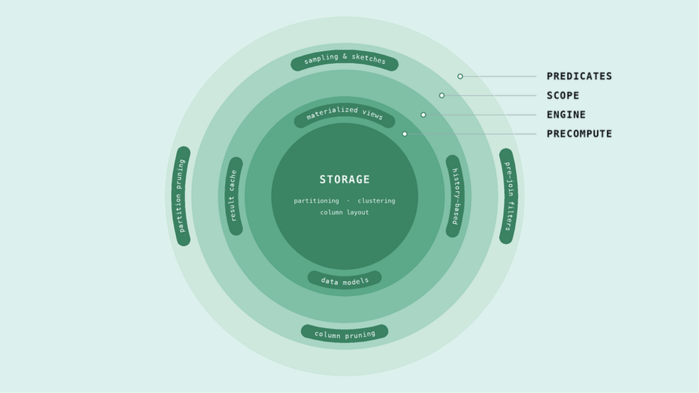
I call them the five layers of BigQuery query optimization:
Each layer gets before-and-after examples and a way to measure it yourself. The techniques mapped to each are non-exhaustive; more can be added as you refine your architecture and as BigQuery ships new features.
If you slice the circular cover image as it becomes a flat table, we can clearly visualize each of the optimization layers and how much each technique affects the other.
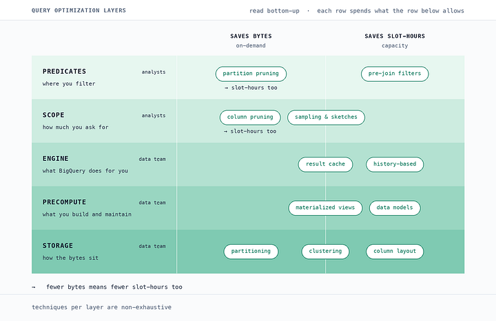
In this article we will walk these layers from the outside in: from the layers where most people spend their time until we reach the storage one that decides whether any of the outer ones are possible. Keep this value ordering in mind as you read this article, because it runs almost exactly opposite to the effort ordering.
First, the techniques divide by the resource they save: bytes for On-demand, slot-hours for capacity. Some sit on the boundary, because fewer bytes scanned means less data for an aggregate to work with.
Second, ownership dictates execution. The outer Predicates layer is a free-for-all populated by analysts, dbt models, BI tools and now AI agents. The foundational layers (Engine, Precompute and Storage) are usually governed by the data engineering team.
That gives us a law for BigQuery query optimization, based on our model: inner layers set the ceiling, outer layers spend it. Let’s look at what this can mean in practice. For instance, trying to prune data in a WHERE clause saves nothing on an unpartitioned table. Column pruning is hard-capped by the physical byte layout of the columns themselves. An extreme example of this is that if you have only one deeply nested JSON column, you will not get any benefits of columnar layout and pruning. The deeper you go, the harder the change is to deploy: a predicate change at the edge is a pull request, modifying a clustering key at the core is a table migration.
Let’s start at the very edge, and work inwards.
The outermost edge. Cheapest layer to change, most familiar to analysts, and the only layer most generated SQL ever touches. Because everyone has access to the WHERE clause, it is also where myths are created.
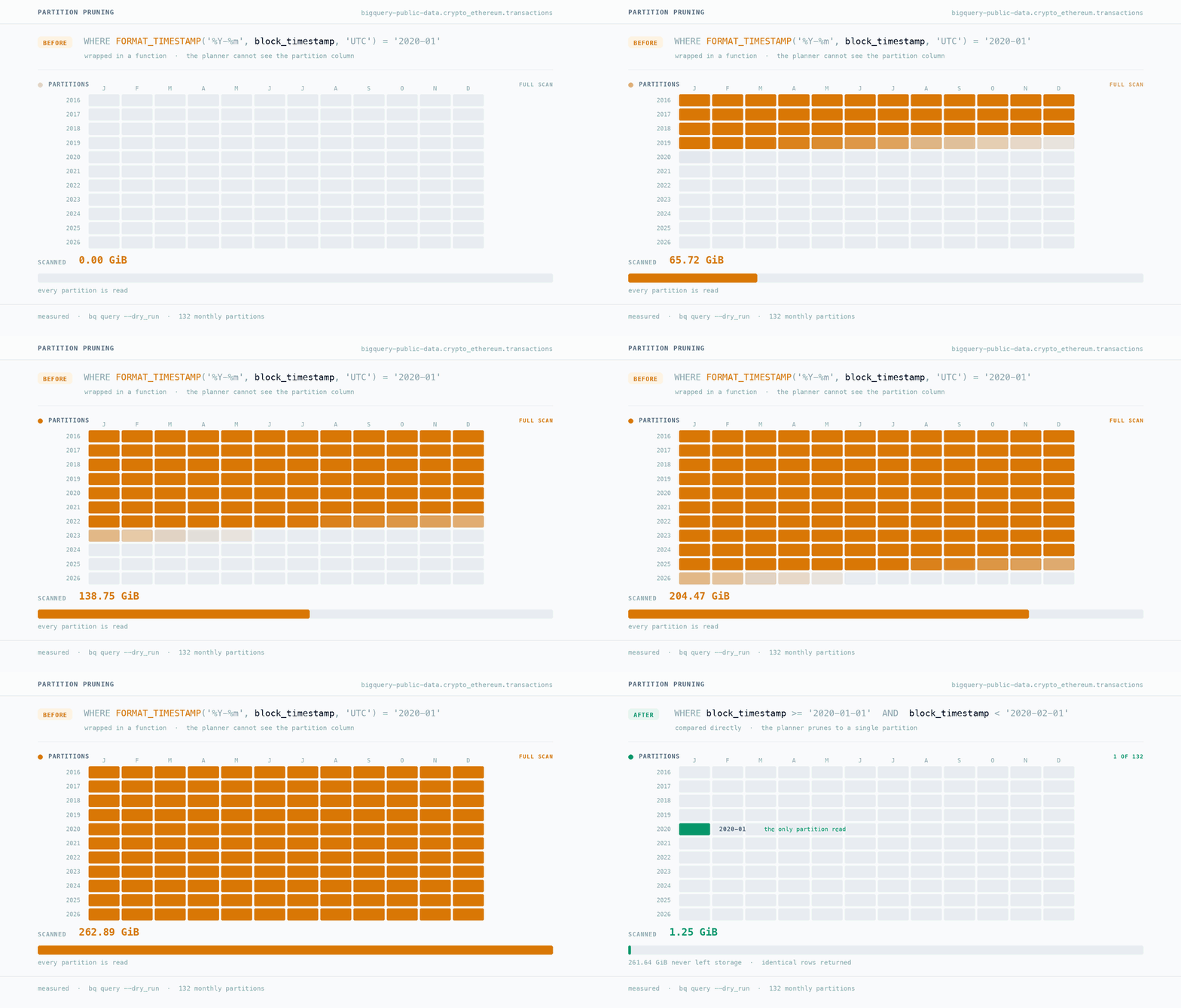
A partitioned table only saves you money if BigQuery can work out which partitions it needs at planning time. Everything that defeats pruning does so for one reason: if the planner is forced to execute logic per row to find the partition, it scans the entire table.
The Anti-Pattern: Defeating the Planner
-- Blocks pruning: the function must be evaluated per row
SELECT * FROM `bigquery-public-data.crypto_ethereum.transactions`
WHERE FORMAT_DATE('%Y-%m-%d', block_timestamp) = '2020-01-01'
Because a function is wrapped around the partition column, the planner is blind. It cannot know the result without reading the row first, so this triggers a full scan: BigQuery reads all 132 months to find the single day you asked for.
The Fix: Clean Pruning
-- Prunes cleanly: identical rows returned, planner sees the literal bounds
SELECT * FROM `bigquery-public-data.crypto_ethereum.transactions`
WHERE block_timestamp >= '2020-01-01'
AND block_timestamp < '2020-01-02'
Both return the same rows. Because the second compares the partition column directly against literals, the planner discards every other partition before reading a byte.
Isolating the partition column on one side of your operator is the gold standard, but BigQuery does not always force raw literals. The planner accepts a whitelist of built-in functions and formats (docs): with constant secondary arguments it prunes through DATE_TRUNC, TIMESTAMP_ADD and EXTRACT, and it parses FORMAT_TIMESTAMP with exact specifiers like %Y-%m-%d. Step outside that whitelist and the optimization breaks silently. The docs support %Y-%m-%d for FORMAT_TIMESTAMP, which leads many to assume FORMAT_DATE behaves the same way. It doesn’t.
Never assume the engine will figure it out for you. BigQuery is full of small gotchas, trust me. Use a dry run to verify your WHERE clause is actually pruning bytes.
Pre-join Filters
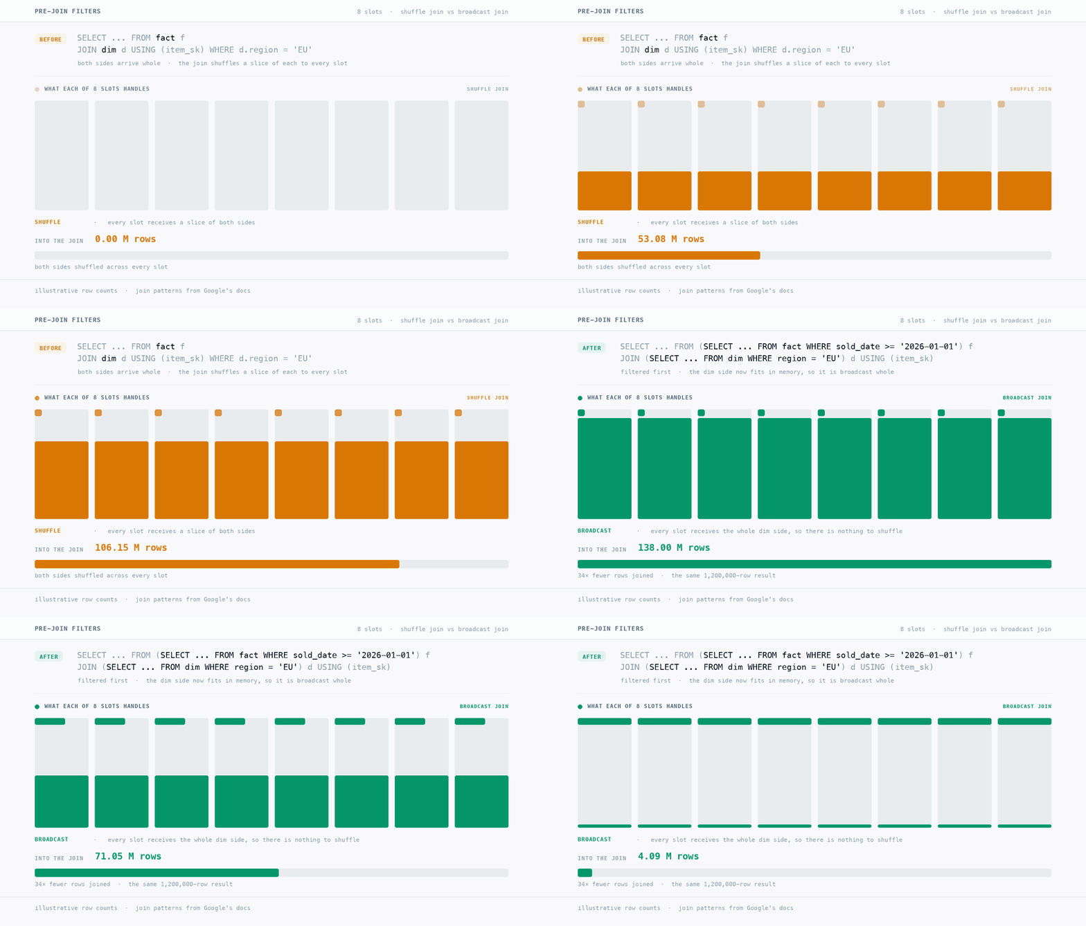
Filtering before a join is usually sold as “fewer rows are cheaper”. True, and it misses the point: the real goal is dropping one side under the broadcast threshold. Feed 138 million rows into a join, as in the animation, and BigQuery defaults to a shuffle join, redistributing both sides across every slot so matching keys land together, moving enormous amounts of data across the network. Pre-filter one side far enough and it flips to a broadcast join, replicating the small side to every worker instead, and network movement drops to near zero.
BigQuery's own optimizer is awake, though. The myth says to always pre-filter in subqueries, which implies it does nothing. BigQuery uses predicate pushdown, moving filters as close to storage as possible before data is retrieved, so on a standard INNER JOIN rewriting a plain WHERE into subqueries frequently changes nothing.
Manual pre-filtering earns its keep only where the planner cannot push down by itself:
Miss one and all 138 million rows go straight into that shuffle.
Which columns you pull and how many rows you request. Both are declared explicitly by you, billed before the engine runs the query, and visible in a dry run, which makes Scope the cheapest layer to verify.
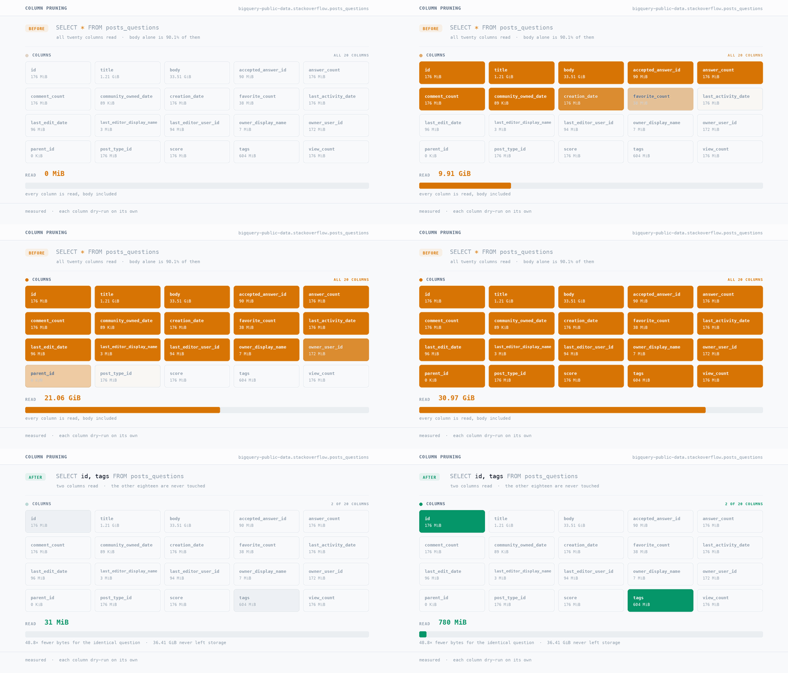
The animation above profiles bigquery-public-data.stackoverflow.posts_questions. A query for two columns against a lazy SELECT * is nearly 50 times fewer billed bytes for the same answer.
What the visual makes obvious is how unequal the columns are. Dry-run all twenty individually and one text column, body, turns out to be 90.1% of the table’s physical footprint.
SELECT * is rarely expensive because it reads twenty columns. It is expensive because it drags that one massive column along for the ride. Before you burn hours rewriting forty queries to trim a few lightweight INT64 fields, find your table’s body column first.
The complex type trap. BigQuery’s columnar storage prunes native STRUCT fields, so querying nested_col.single_field only pays for that leaf. You pay for the whole structure if you SELECT nested_col at the root, or if the data is JSON, where extracting one key forces a full scan of the string.
LIMIT is an illusion. LIMIT 10 restricts what is returned to your screen, not what is read from disk. Adding it on the end of a SELECT * does nothing to reduce bytes scanned.
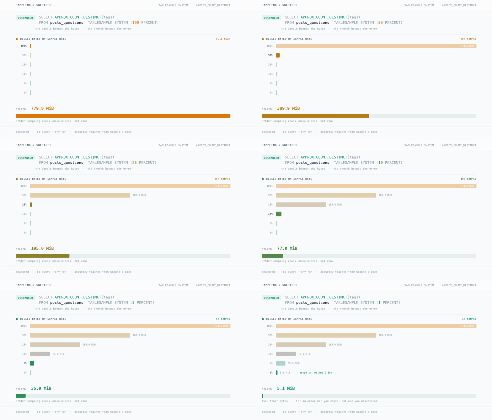
If LIMIT does not make querying cheaper, BigQuery offers two options that do, balancing precision against performance and cost. They are distinct techniques used for different reasons.
TABLESAMPLE: bounding the bytes. As the animation shows, a sample rate reduces the bytes read from disk in proportion to the rate you ask for. At the low end it does better than proportional: ask for 1% and you might be billed for 0.66%, because SYSTEM sampling reads whole randomized blocks rather than individual rows.
Why use it: Discovery, and the development loop. Nobody re-runs a finished, perfect query twenty times, but everybody re-runs the one they are still writing. Or the one to check the schema, even though they shouldn’t.
Sketches: bounding the error and the compute. Where sampling restricts how much data is read, a sketch restricts the CPU and memory needed to aggregate it. BigQuery uses HyperLogLog++ for distinct counts and KLL for quantiles, available on wrappers like APPROX_COUNT_DISTINCT. Sketches can also be extracted, stored in a table and merged later, turning a repeated full-table aggregation into a cheap re-aggregation.
Why use it: production reporting where exactness is not necessary but speed is. Note: a sketch saves compute, which a dry run cannot show you.
Free, automatic and hands-off. You cannot configure these; you can only write queries that use them or, quite easily, queries that break them.
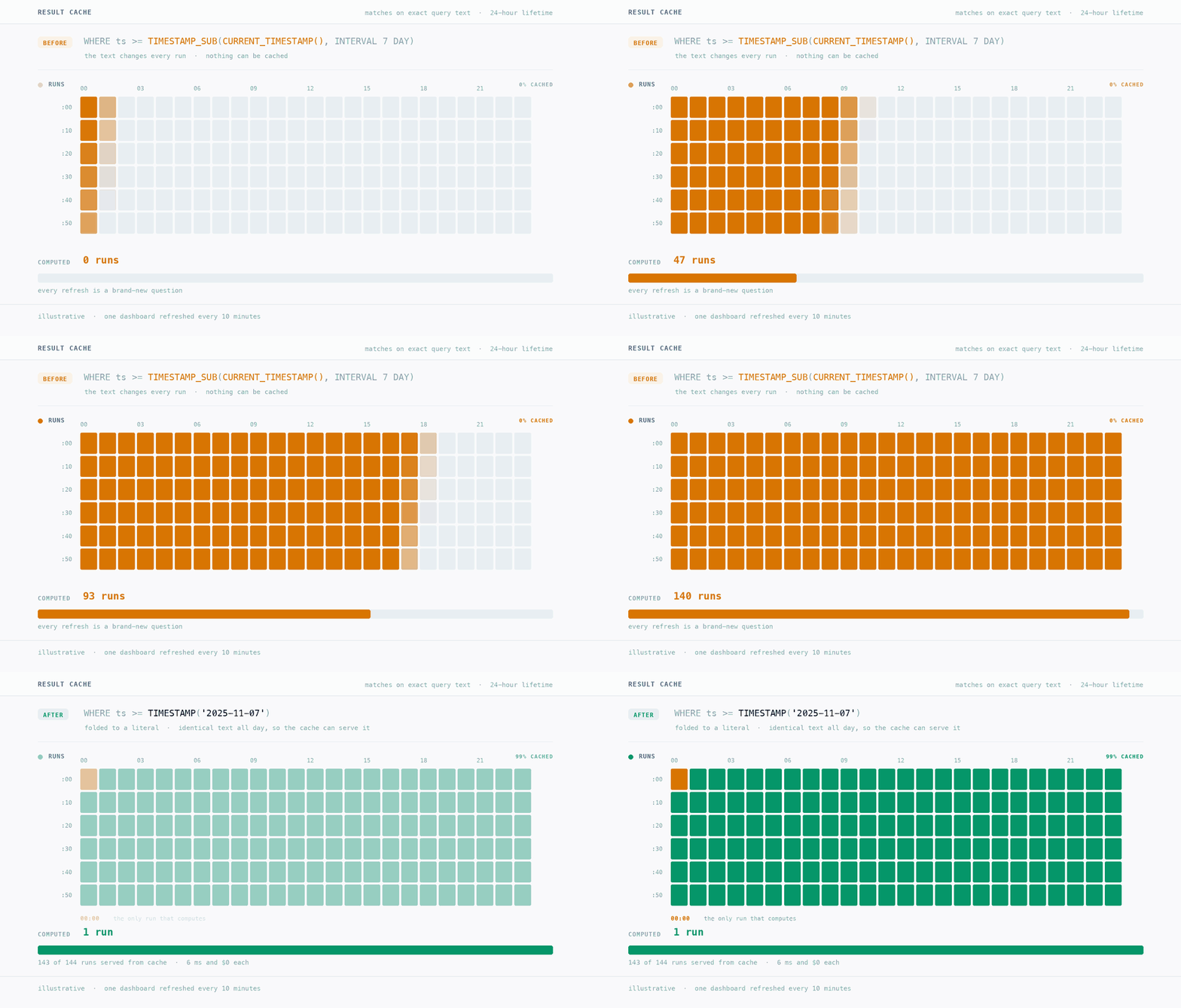
The result cache is free, instant, and stores results for 24 hours, under strict rules: it matches on exact query text and refuses to cache any query containing a non-deterministic function such as CURRENT_TIMESTAMP() or CURRENT_DATE().
The dashboard trap. Combine a frequent refresh rate with a non-deterministic function and you get the most expensive habit in the BI world. A query like WHERE event_date >= DATE_SUB(CURRENT_DATE(), INTERVAL 7 DAY) rewrites its own text every time it runs, so BigQuery treats each execution as a brand-new question: one dashboard refreshing every 10 minutes, 144 runs in a day, not one of them cached.
Resolve that expression into a hardcoded date literal in your semantic layer and the query text becomes static. You pay for the first run; the next 143 hit the free cache. This is not always possible, because these queries are usually auto-generated by BI tools.
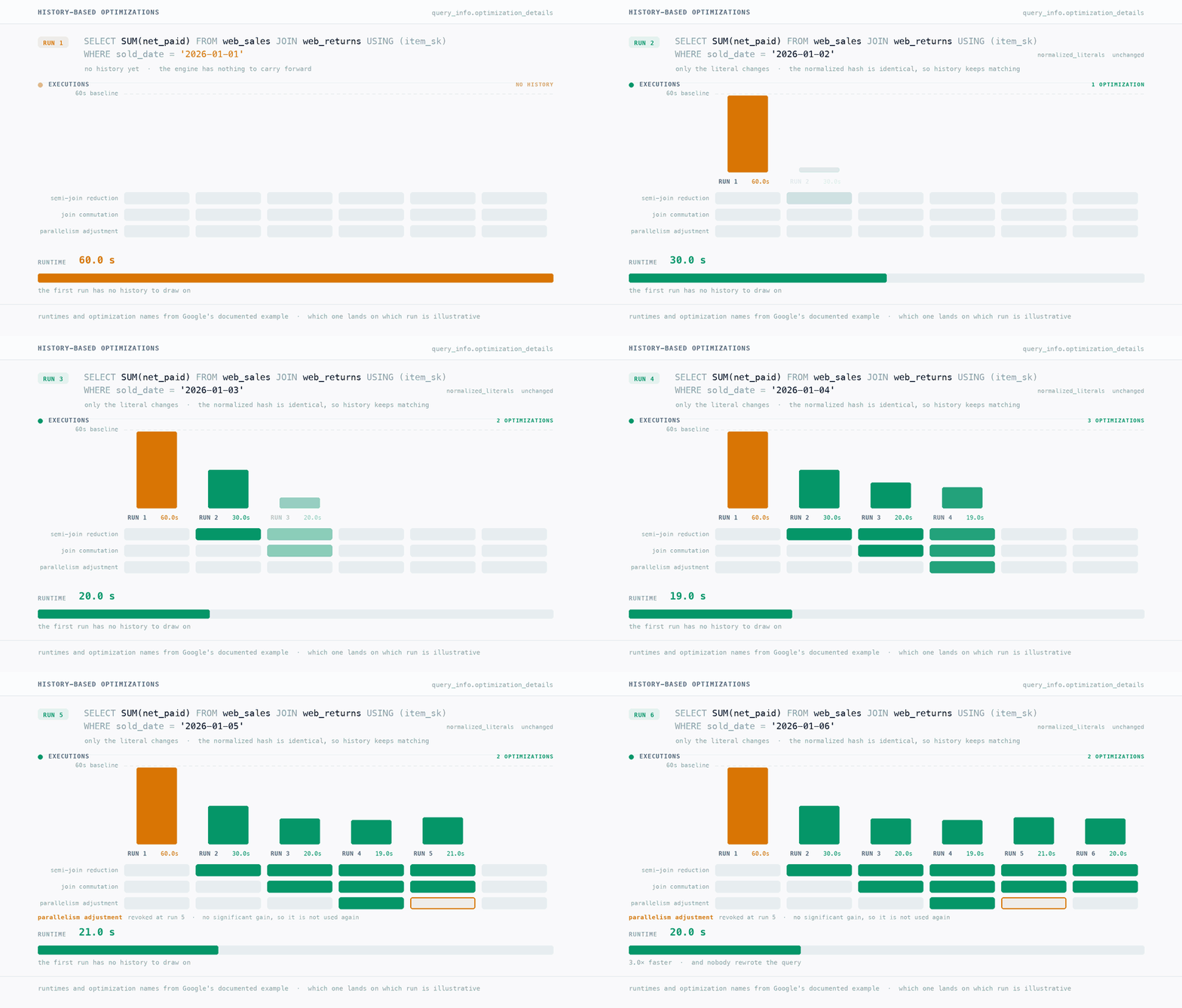
Just like humans, BigQuery can learn from its past. The animation shows a query starting at a 60-second baseline with no history. Over subsequent executions the engine applies learned optimizations in sequence: a semi-join reduction, then a join commutation, then a parallelism adjustment, driving execution down to 15 seconds.
It does this by retaining execution metrics from completed runs of the same or “similar” queries. Similar means the engine hashes the query text but normalizes the literals, so a query filtering event_date = ‘2026–09–10’ produces the same hash as event_date = ‘2026–09–11’. That matters: history-based optimization survives dynamic date filters, where the exact-match result cache fails immediately. It requires repetition, so a workload of one-off queries never builds the history to benefit, and it is self-correcting: if an optimization makes a run slower, BigQuery withdraws it.
Configuration and impact. History-based optimizations are on by default, and Google keeps adding strategies behind the scenes with no code changes on your end. Leave it on. You do not have to guess how well it is working: there is a sample query that ranks your queries by estimated improvement.
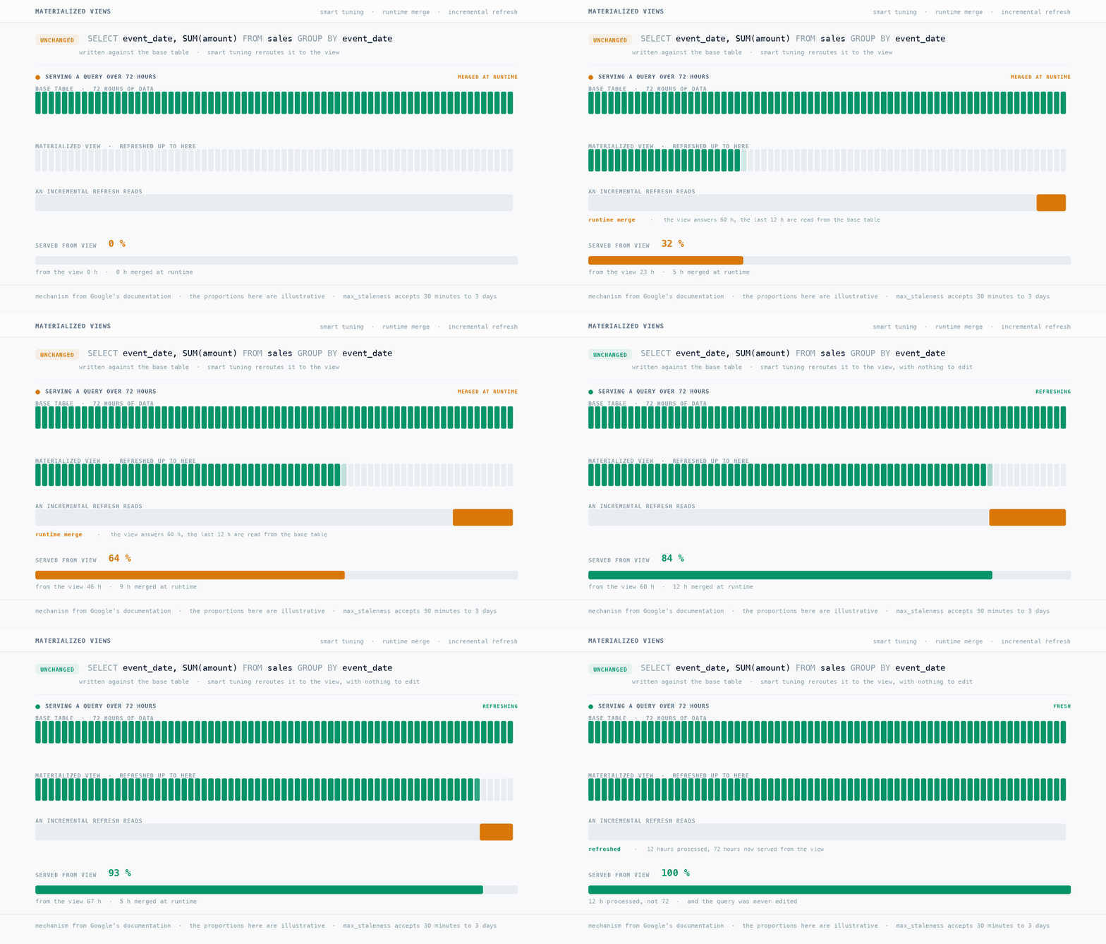
With materialized views your underlying SQL does not change. If any part of a query against a base table can be answered more efficiently by an existing view, BigQuery reroutes it automatically.
The runtime merge. The animation breaks down a base table holding 72 hours of data alongside a view refreshed up to a point in time. BigQuery reads the bulk of the answer from the view and only scans the base table for the un-merged delta. Served as view plus delta, a materialized view can cut billed bytes while never serving a stale result.
Refreshes and staleness. When the view updates it reads only the newly arrived data instead of doing a full-table scan. You control how often that background compute happens with max_staleness, which accepts 30 minutes to 3 days, trading freshness against refresh cost.
The edition constraint. One catch turns this into a FinOps decision rather than a technical one: you cannot create materialized views on BigQuery Standard edition. You need Enterprise, Enterprise Plus, or the On-demand model.
Data modeling is not a BigQuery problem; it is the fundamental work across any analytical database, and how to do it well fills whole books. What this section covers is the narrow part that matters for cost: what you actually trade when you widen a table, and why the choice sets the ceiling on everything above it.
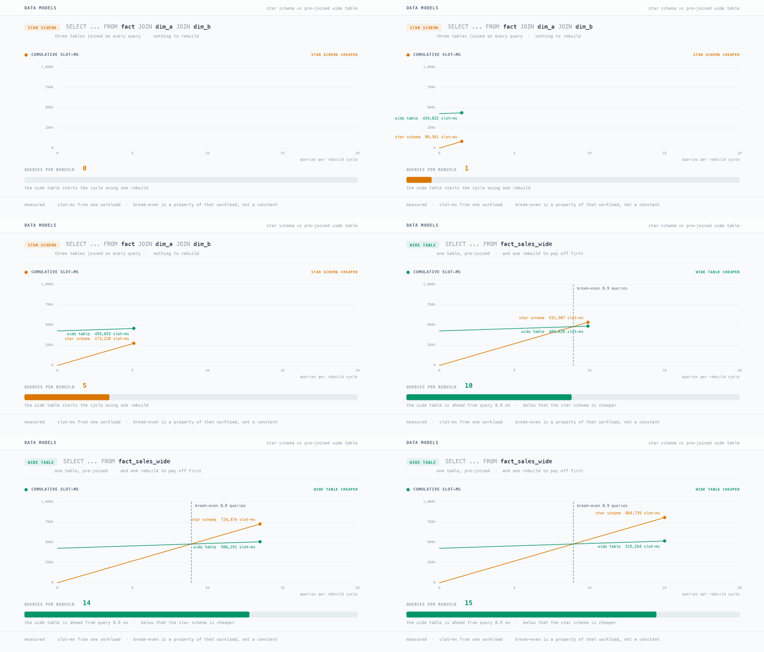
Wide tables are fine, and the columnar defense is real. BigQuery only reads the columns you name, so the columns nobody touches cost nothing. The SQL gets simpler for whoever is consuming it. For data that is read a lot, the read-side win shows up in the numbers: in one example we measured, joining three tables was 8.9 times more expensive in slot time than reading the same rows pre-joined into one wide table, and 15% more in bytes scanned. Most advice stops here and tells you to denormalize.
The unit of account is the refresh cycle, not the query. One rebuild costs more than any single query against it saves. You have to run enough queries to pay it back. In the example above the break-even is around 9 queries per rebuild cycle on slot time, and 14 on On-demand bytes. Below that the joined version is cheaper. The useful conclusion is not "denormalize above 9 queries". It is that joins cost less than their reputation suggests, and the gap is small enough that it should not be deciding your data model for you.
What actually costs you is the refresh graph. Everyone warns about storage duplication. Columnar compression absorbs almost all of it, about 1.1% growth, pennies a month. The real bill is lineage. If everything lives in one wide table, changing one column rebuilds all of it. A 10% improvement on a query does not mean much when a single model change triggers a full refresh of the whole warehouse. Schema changes and backfills stop being normal.
Split your models by how often they change. If you already run something like medallion or staging/intermediate/marts, you have the shape: layers, with reads only flowing downstream. People usually argue about models in terms of how maintainable the code is, but layers matter for cost too. Merge two layers together and any change to either one now rebuilds both. Keep them apart and the work stays local: what you touched and whatever depends on it, not the whole warehouse.
One useful distinction is between rows that record something and rows that infer something. At Alvin we dogfood our own product on BigQuery, and this was the split that mattered most when we remodeled: an observed layer (cleaned and conformed, one row per thing that happened) and a modeled layer on top of it, where our interpretation lives. Observations do not get revised often, but our models change every time our logic does. In one table, every modeling change reprocesses the history too. Splitting does ask more of you: it means being deliberate about grain, and every new grain is one more place where the numbers can be wrong without anyone noticing.
The takeaway: start normalized, enough to keep your entities and their grain distinct, and widen at the consumption edge. Do it per grain, never across grains. There is a temptation to flatten everything for read speed but the additional compute may not pay off.
The core of that initial figure is physical preconditions: partitioning, clustering, and how the bytes are distributed across your columns. Every optimization discussed so far is capped by these fundamentals. Column pruning on a table where bytes are spread evenly saves a little margin.
On the table we looked at earlier, one text column dominated the footprint, and pruning it was worth nearly 50 times the bytes. Clustering picks up where partitioning stops: it sorts rows within each partition so a filter on a high-cardinality column skips blocks instead of reading them. Its savings never show up in a dry run, because the estimate is computed before block pruning happens, which is why people often conclude it did nothing. Fixing these choices requires DDL changes and backfills, which is why enabling require_partition_filter is not a minor SQL tip but a governance policy that belongs at the storage layer.
If your architectural ceiling is broken, no amount of clever SQL rewriting bypasses it.
In most production environments the most expensive SQL is not written by a human. It is generated by Looker, by dbt macros, by a semantic layer, and increasingly by AI agents with a BigQuery connection and no clue how much their queries cost.
That generated SQL only ever touches the outermost layers. A BI tool cannot choose a materialized view, it will not resolve a dynamic date function into a static literal, and it has no opinion on how your tables are partitioned.
You cannot send a code review to a BI tool. Sometimes you can optimize a LookML definition, if you own the repository and know which of the several hundred files is responsible. Mostly you cannot.
Hand-optimizing generated SQL is an endless battle that accelerates every time someone publishes a new dashboard, and you can never optimize fast enough to keep pace with a business whose data is growing, especially in this agentic era we live in.
Instead of fighting symptoms at the outer edges, shift focus to the structural foundation.
Audit cache hits with dollars, not percentages. A 50% hit rate on thousands of tiny UI dropdown queries saves pennies; focus on the heavy analytical queries missing the cache.
Neutralize the dashboard trap. Find your most expensive, frequently refreshed dashboard and push the dynamic date logic into your semantic layer (when your BI tool allows it), so BigQuery receives static, cacheable literals.
Force the issue on storage. List the ten largest tables being scanned without a partition filter and enable require_partition_filter on the heaviest offender.
Protect from the column heavyweights. Restrict SELECT * in your queries, find your most expensive queries and dry run against their largest referenced tables, and find whether a massive text or JSON field is being dragged through every lazy query.
The performance ceiling of your warehouse is dictated by the physical layout of the bytes on disk and the models sitting on top of them. Stop trying to out-query a bad architecture.
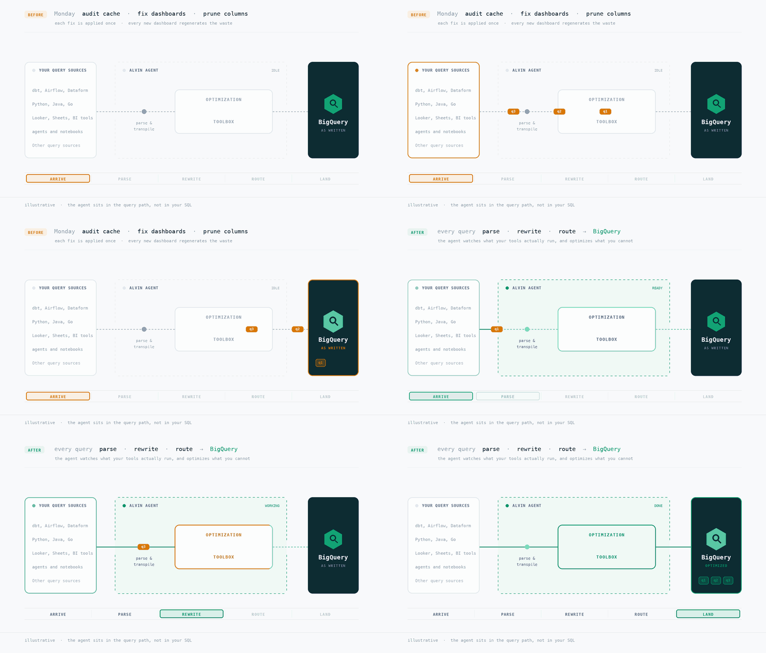
Everything above is a one-time fix applied to a system that regenerates its own waste every time someone builds a dashboard or adds a new pipeline.
Every layer in that stack breaks on its own. A predicate gets dropped when someone refactors a dbt model. Scope widens when a BI tool adds a column to a dashboard. The result cache stops hitting the day a timestamp enters the WHERE clause. A workload stays on the edition it was first placed on, long after the break-even moved. None of this announces itself: the query still returns the right answer, it just costs more, and the bill arrives a month later with no attribution attached.
That is the problem we work on at Alvin, the automated BigQuery cost optimization platform: watching the queries your tools actually run, ensuring you are getting the best of any query optimization you have applied, and optimizing it for you when you cannot. Partition filters you never wrote, cache rewrites applied for you, each workload routed to the pricing model it actually belongs on, and more landing in Alvin’s optimization toolbox all the time!